Before diving into a discussion of genomics and natural language processing (NLP), we should review a basic primer of molecular biology. For the biologists out there, forgive me for making some oversimplifications. This field is much richer than can be fit in one paragraph! And for the computer scientists out there, there really is more to biology than dissecting frogs and annotating oversaturated printouts of the endoplasmic reticulum.

Molecular biology primer

DNA is the “blueprint” of the human body that holds our genetic code. Every cell in a specific organism possesses identical DNA (barring mutations that accumulate over a person‘s life); it is regulation of this DNA that leads to differences between cell types (eg neuron vs. liver cell). DNA is a large molecule comprised of nucleotides — small chemical subunits that can be abstracted as “letters”. These four nucleotides are adenine (A), cytosine (C), guanine (G), and thymine (T). DNA is packaged into chromosomes. Humans have 46 chromosomes and are diploid — our chromosomes come in pairs, where we inherit half of our chromosomes from our mom and half from our dad. The chromosomes are numbered 1-22 (autosomes — descending order of length) and X/Y (sex chromosomes). The human genome contains ~3.2 billion nucleotides in total. The central dogma of molecular biology describes the fundamental role of DNA: DNA is transcribed into messenger RNA (mRNA), a form of ribonucleic acid (RNA), and mRNA is translated into protein. Only ~1–2% of DNA encodes mRNA; the rest of DNA is involved in regulation of gene expression, transcription into non-coding RNA, structural roles (such as centromeres and telomeres), has uncharacterized function, or may serve no function at all. mRNA is also comprised of nucleotides like DNA, and is grouped into triplets called codons during translation, where each codon encodes an amino acid. Amino acids are the subunit of proteins. There are 20 amino acids (the memorization of which is a rite of passage for every biochemistry student), each characterized by different chemical structures and properties (e.g., polarity, acidity, size, disulfide-bond potential, phosphorylation potential). As there are \(4^{3} = 64\) possible nucleotide combinations in a codon, the existence of only 20 amino acids implies that the genetic code is degenerate: 1-4 codons will encode the same amino acid. Proteins do the work of the cell — they catalyze reactions, communicate signals, transport molecules, build structures, and much more. Effectively, DNA is relevant only insofar that it encodes mRNA, which itself encodes protein — DNA molecules themselves serve essentially no role in the human body outside of this function.

DNA and NLP similarities and differences

At first glance, genomics looks like a direct analog to natural language processing. And in some respects, it is. Both the English language and the genetic code share a small finite alphabet — English has 26 letters, and DNA has four nucleotides (ACGT). Both have an exponentially large number of units that can be formed by unique permutations of this alphabet — English groups letters into words, and DNA groups nucleotides into genes. The two vocabulary sizes are comparable — there are ~20,000 words in the English language and ~20,000 genes encoded in the human body.

But there are also some crucial differences that must be addressed. For instance, English words are often within a narrow length range of 2 to 10 characters. Genes, however, range anywhere between 1,000 to 1,000,000 nucleotides. Changing an English sentence with even a single letter substitution is guaranteed to change the meaning of a sentence, as the similarity in meaning between words holds minimal correlation with similarity in structure. With DNA, some base substitutions are completely invisible, some have modest effects on outcome, and some are catastrophic. Mutations outside gene-coding regions nearly always have no effect. Mutations within gene-coding regions generally only have an effect if they cause a change in amino acid, and especially if they significantly change the chemical properties of the amino acid. Mutations are significant when they result in a change in protein folding structure, which can lead to protein instability or loss of ligand specificity.

DNA and English text also have different numbers of hierarchical groupings. As discussed earlier, nucleotides can be thought of as analogous to letters, and genes can be thought of as analogous to words. Carrying forward this analogy, each chromosome or entire human genome could be thought of as analogous to a document. However, there is no analogue to a “sentence” for DNA. Each “document” would simply read as a list of words used exactly one time, likely ordered based on their position in the genome — an order that has little functional significance. Or, perhaps, different conventions can be applied to DNA. For instance, an alternative representation would be to represent DNA codons as letters, rather than individual nucleotides, which would create a 64 character alphabet rather than a four character alphabet. This would pose its own challenges, however, such as the degeneracy of the DNA code (up to four codons can encode the same amino acid, with the last nucleotide often being flexible) and the questionable relevance of codon-tokenization in non-coding regions (where transcription does not occur). Or, alternatively yet again, if we stick with nucleotides as letters, then these codons or other k-mers (subsequences of length k) could represent words, and genes could represent sentences. But this still runs into the problem of high “sentence” similarity and “document” structure.

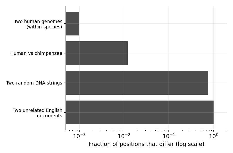
Any two English sentences or documents will contain vastly different structure. Some documents might be one sentence, while others might be hundreds of pages long. The lengths of sentences and vocabulary used can vary widely. For text classification, such as sentiment analysis, the entire body of text must be analyzed, as each portion can contribute to the meaning of the text as a whole. In contrast, DNA has a highly consistent structure between individuals. Any two individuals are ~99.9% identical. Of the ~3.2 billion nucleotides in the human genome, only ~10 million nucleotides have substantial (common) variation across the human population¹. This shallow diversity is due to a population bottleneck approximately 50,000 years ago which restricted our genetic ancestors to approximately 10,000 individuals. Most of these variants have a most common form, which can be collected into what is called a reference genome¹. In addition to these ~10 million sites of possible variation, each person has ~70 de novo mutations that are specific to them³, and any given cell may accumulate up to several thousand somatic mutations over the person’s life⁴. This means that any artificial intelligence (AI) model that ingests the entire 3.2 billion nucleotide sequence is exerting a lot of unnecessary energy, as most sites are essentially guaranteed to match the reference genome. There are benefits to working with raw DNA sequences as well. The simplicity of the input data, the direct analog to natural language, and the ability to maintain the full context of DNA that is especially relevant for tasks such as mutation effect prediction. But this trade-off is unique to genomics data and should be intentionally considered by the machine learning practitioner.

Figure 1: Two members of the human species are near-duplicates. The fraction of positions that differ between two sequences, on a log scale: two humans differ at only ~\(10^{-3}\) of positions and human versus chimpanzee at ~\(10^{-2}\), whereas two random DNA strings differ at \(0.75\) and two unrelated English documents at essentially every position. The within-species genomic “corpus” is roughly a thousandfold more redundant than text.

Sources of genomic data

Genomics data can come from multiple sources. These include whole genome sequencing (WGS; sequencing the entire genome), whole exome sequencing (WES; sequencing only the gene-encoding regions of the genome), bulk RNA-sequencing (bulk RNA-seq; sequencing all expressed RNA), and single-cell RNA sequencing (scRNA-seq; sequencing RNA at single-cell resolution). These sequencing machines have ~99–99.9% per-base accuracy. When only mildly confident about the detected nucleotide, the machine may report a lowercase letter. When entirely unconfident, the machine may report an “N”. How to handle these additional characters is a design decision in any tokenizer.

The protocol to sequence genomic data depends on the assay and technology, but they all share the isolation of genetic material, decomposition into small regions generally between 75-150 nucleotides (reads), amplification by polymerase chain reaction (PCR), and sequence readout. The reads (FASTQ file) are usually mapped to the reference genome (FASTA file) to produce a genome alignment (BAM, or Binary Alignment Map, file). For DNA, the variants can be extracted in a VCF (Variant Call Format) file. For RNA data, the count of each gene can be stored in a count matrix, where each row represents a sample (bulk RNA-seq) or cell (single-cell RNA-seq), and each column represents a gene.

DNA, RNA, and protein

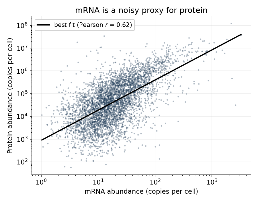
I mentioned earlier that proteins are the real molecule of interest in the human body, so why do we measure RNA at all rather than measuring protein directly? One of the main reasons is that protein sequencing technology has simply lagged behind nucleotide sequencing technology in cost. The underlying assumption is that RNA levels correlate strongly with protein levels, so the former can be used as a proxy for the latter. However, this may be a stronger assumption than most would like to believe. Across many careful studies, the correlation between a gene’s mRNA level and its protein level is moderate at best — typically a Spearman \(\rho\) in the 0.4-0.6 range, and lower still when you look at changes over time rather than steady-state across genes. Schwanhäusser and colleagues found mRNA explained well under half the variance in protein abundance⁵; Vogel and Marcotte, Liu, Beyer and Aebersold, and Buccitelli and Selbach all converge on the same message — translation rates, protein half-lives, and post-translational regulation drive a large share of protein levels that mRNA simply does not see^6–8. Edfors and colleagues showed the relationship is gene-specific⁹: each gene has roughly its own mRNA-to-protein conversion factor, so a single global model is wrong per gene. Figure 2 shows the consequence in real data — even at the optimistic end of that range, knowing a gene’s mRNA leaves its protein level uncertain across a wide band.

Figure 2: mRNA is a noisy proxy for protein. Real per-gene mRNA and protein copy numbers in mouse NIH3T3 fibroblasts (Schwanhäusser et al. 2011; \(n=4{,}309\) genes; Pearson \(r=0.62\) on log abundances). The red line is the best fit; even so, protein scatters across two to three orders of magnitude at any given mRNA level, because translation and degradation are not observed in the RNA.

Popular datasets

Below is a set of some of the most popular public datasets in genomics. File sizes can be quite large — for WGS, FASTQ files are often around 100-200GB, BAM files are 30-100GB, and VCF files are 1-10GB. However, as described earlier, much of this information represents redundancy with the reference genome, and individuals are often the unit of interest when training AI models rather than nucleotides, so cohort sizes in the thousands-hundreds of thousands range is often fairly small for modern AI. Additionally, most data are collected on healthy individuals or individuals with cancer, so it is difficult to study other diseases because public datasets will be quite small (if available at all). And any data collected from a single institution or region will have batch effects, limiting generalizability to other populations.

Assay abbreviations: WGS = whole-genome sequencing; WES/WXS = whole-exome sequencing; bulk RNA-seq = bulk RNA sequencing; scRNA-seq = single-cell RNA sequencing; Array = genotyping microarray; WSI = whole-slide imaging; ChIP-seq = chromatin immunoprecipitation sequencing; ATAC = assay for transposase-accessible chromatin; DNase = DNase I hypersensitivity sequencing.

Two structural problems run underneath these numbers.

How real models approach this

We’ve talked a lot about how genetic material can be represented as text for AI models. But what is actually done in practice? Here are a few notable examples.

• AlphaFold2 (Jumper et al.²²) predicts protein three-dimensional (3D) structure from amino-acid sequence at near-experimental accuracy — arguably the field’s defining success. It takes a protein’s amino-acid sequence, together with a multiple-sequence alignment of evolutionarily related proteins and any available structural templates, and predicts the 3D coordinates of every atom. The sequence is treated as a string over the fixed 20-letter amino-acid alphabet — each residue is mapped to a learned embedding rather than an arbitrary text token — and much of the biological signal comes from the MSA, whose column-wise evolutionary covariation encodes which residues are likely to contact one another in 3D. Protein folding is a problem that possesses multiple attributes that make it an ideal candidate for AI. The 3D structure depends entirely on the discrete amino acid sequence itself, without dependencies from other parts of the genome or cell state broadly. There are over 200,000 experimentally determined protein structures with resolved amino-acid sequences across humans and model organisms²³, representing a dataset that is large enough for supervised learning. And amino acids have biochemical properties that enable logical verification of predicted results to an extent.
• Enformer²⁴ and AlphaGenome²⁵ attack the cis-regulatory problem head-on, predicting expression and chromatin readouts from sequence across ~200 kilobases and up to 1 megabase windows respectively. They are the state of the art on long-range cis effects — and structurally blind to trans regulation that acts through diffusible proteins or other chromosomes. Both take a one-hot-encoded DNA sequence — a long genomic window centered on the region of interest — and predict thousands of functional genomic and epigenomic tracks (expression, chromatin accessibility, histone marks, and more) along that window. Here the alphabet is simply the four DNA bases (A/C/G/T): each position becomes a 4-dimensional one-hot vector, so — unlike a text model with a learned subword vocabulary — there is no tokenization step at all, and biology enters through the fixed base alphabet and the reverse-complement symmetry the architectures are built to respect (a sequence and its complementary strand should give the same prediction).
• DNABERT²⁶, the Nucleotide Transformer²⁷, and Evo²⁸ are DNA “language models” — masked or autoregressive pre-training over genomic sequence, transferred to downstream tasks. Each tokenizes raw nucleotide sequence — overlapping k-mers for DNABERT, fixed non-overlapping k-mer tokens for the Nucleotide Transformer, and single-nucleotide (byte-level) tokens for Evo — and learns representations by predicting masked or next tokens over large genomic corpora. The vocabulary is built from the four nucleotides rather than natural-language words, and the differing tokenizations are attempts to package that four-letter alphabet into biologically meaningful units: k-mers approximate short motifs or codon-like chunks, while single-base tokens keep every nucleotide addressable at the cost of longer sequences.
• scGPT²⁹ and Geneformer³⁰ bring the foundation-model recipe to single-cell transcriptomics, learning representations of cell state from large RNA-expression atlases. These approaches do not take in raw sequencing reads as input, but rather the processed count matrices. Consequently the “alphabet” is not sequence at all but the roughly 20,000 genes — each gene is a token, and its expression level is encoded either by binning the count into discrete value tokens (scGPT) or by ranking genes from most to least expressed within a cell (Geneformer), so the biology is carried by which genes are on and their relative levels rather than by any letter sequence.

Conclusion

There have been exciting developments in genomics AI, and there is much to be done moving forward. ~40% of variants in cancer cases are still classified as variants of unknown significance³¹. When analyzing a cancer patient’s mutations, it is still often impossible to distinguish the driver mutation from passenger mutations. The role of genomics outside of cancer and well-characterized genes characterized by single mutation/gene events is minimal in clinical practice. A single human scRNA-seq experiment often has thousands of cells, and tens of thousands of genes. In an atlas comprised of dozens or hundreds of datasets, there can be millions of cells, with various sources of batch effects. Continuing to develop models that can make sense of these data will be critical for advancing genomics research.

References

Why a computer-vision expert’s intuitions misfire

If you have trained a model on ImageNet, COCO, or a few hundred million Instagram photos, you have excellent instincts for natural-image vision. Most of those instincts are wrong — or at least dangerously incomplete — the moment you point them at a chest CT or a screening mammogram.

This post is a field guide for machine-learning scientists moving into radiology. It is not a survey of architectures; the architectures are mostly the ones you already know (CNNs, U-Nets, vision transformers, increasingly foundation models). What changes is everything around the architecture: the statistics of the signal, the cost and meaning of a label, the data you can actually get, and — the part that quietly sinks most projects — generalization across the bewildering heterogeneity of how medical images are produced. I will end with the two things ML scientists most often discover too late: how the FDA actually regulates these models, and why the model in the paper is rarely the model that ships.

A running theme: medical imaging is in some ways easier than natural-image vision, and leaning on those advantages is the difference between a model that demos well and one that survives contact with a second hospital.

What is genuinely easier than natural images

Start with the good news, because it is real and underexploited.

Canonical pose and framing. A street scene can contain a cat at any scale, any orientation, anywhere in the frame, against any background. A PA chest radiograph is, by protocol, a patient standing upright, facing the detector, arms positioned to rotate the scapulae off the lung fields. The heart is on the left.¹ The aortic knob is where the aortic knob goes. This is a strong spatial prior that natural-image models simply do not get for free — and it is why registration, atlas-based priors, and even fixed positional encodings work far better here than they would on web images.

One channel, calibrated. Most modalities are grayscale, and — crucially — the gray values often mean something physical. CT is quantitative: each voxel is a Hounsfield unit, a linear transform of the X-ray attenuation coefficient \(\mu\) relative to water,

so water is \(0\), air is \(-1000\), fat is around \(-100\), and cortical bone is \(+1000\) or more. Fat is fat in every CT scanner on Earth. Nothing in RGB is calibrated like this; “how blue is the sky” is not a physical constant. You can and should exploit it — windowing, HU-based preprocessing, and physically motivated augmentations all follow from it.

The suspected disease localizes attention. Clinical imaging arrives with a reason for exam. “Rule out pneumothorax” tells you to look at the pleural line; “rule out stroke” sends you to the brain parenchyma and vessels. The organ of interest is usually known, which is a luxury object detection never has.

But each of these advantages has a barb:

• The canonical pose breaks for portable/supine films, pediatric patients, body habitus, and post-surgical anatomy.
• HU calibration drifts with scanner, kVp, and contrast timing (more on this below), and MRI intensities are not standardized at all — a T1 value is only meaningful relative to the rest of that one acquisition.
• “The organ of interest is known” is a trap: incidental findings in the other organs are often what matter most clinically. The lung-nodule model that ignores the adrenal mass at the edge of the field has failed the patient even if its AUC is perfect.

So: use the priors, but treat every one of them as a covariate that can shift.

The needle in the haystack: subtlety and extreme imbalance

Here is the single biggest statistical difference from natural images. In COCO, the object you care about typically occupies a meaningful fraction of the frame. In radiology, the finding is often a handful of voxels in a sea of normal tissue, and the difference between malignant and benign — between call the patient back and see you in two years — can come down to a few millimeters of spiculation or a subtle change in density.

Make it concrete with geometry. A chest CT of roughly \(512 \times 512 \times 320\) voxels at \(0.7 \times 0.7 \times 1.0\,\text{mm}\) contains about \(8.4 \times 10^7\) voxels. A clinically important \(5\,\text{mm}\) pulmonary nodule is a sphere of volume \(\tfrac{4}{3}\pi r^3 \approx 65\,\text{mm}^3\), or about \(134\) voxels. The lesion is therefore

of the volume — roughly one in six hundred thousand voxels. Shrink it to a \(3\,\text{mm}\) nodule and you are at one in three million. Figure 1 puts several findings on the same axis as natural-image objects; note the five-to-six order-of-magnitude gap.

The consequences for an ML scientist are direct:

• Accuracy is meaningless and pixel-wise loss is treacherous. A segmentation model that predicts “no lesion” everywhere achieves \(1 - 1.6\times10^{-6} \approx 99.9998\%\) voxel accuracy. Use overlap and detection metrics built for imbalance — Dice / \(F_1\), where for prediction \(P\) and ground truth \(G\), \(\mathrm{Dice} = \frac{2|P \cap G|}{|P| + |G|},\) free-response ROC (FROC) for detection, and class-balanced or region-based losses (Dice loss, Tversky, focal). The focal loss down-weights the easy negatives that otherwise dominate the gradient: \(\mathrm{FL}(p_t) = -(1-p_t)^{\gamma}\log p_t\).
• Most of the volume is uninteresting, and uninteresting in a structured way. Hard-negative mining, lesion-aware patch sampling, and two-stage candidate-then-classify pipelines exist because uniformly sampling voxels wastes almost all of your compute on obvious lung parenchyma.
• Resolution is not negotiable. Downsampling a natural image to \(224^2\) loses a cat’s whiskers; downsampling a CT slice can erase the lesion entirely. The signal you are hunting may be at the Nyquist limit of the acquisition.

Annotation is the bottleneck, not the model

In natural-image land, labels are cheap: crowdworkers draw boxes, and “is this a dog” needs no credential. Radiology inverts this completely, and it reshapes what is feasible.

A bounding box is the wrong primitive, and often impossible. Many findings have no crisp boundary. Where exactly does a ground-glass opacity end and normal lung begin? What is the bounding box of diffuse interstitial disease, or of “the lungs look hyperinflated”? The pathology is frequently a texture or a global property, not a localizable object. Even when a lesion is discrete, it lives in 3D — a box becomes a volume, and a radiologist scrolling 320 slices to contour a tumour is spending clinical time that costs orders of magnitude more than a crowdworker.

Ground truth is noisy and sometimes unobtainable from the image alone. The honest label often is not in the pixels. Is that lung nodule malignant? The image cannot say; you need the biopsy, or two years of follow-up showing growth. This is why so many “labels” in public datasets are actually NLP-extracted from the radiology report (MIMIC-CXR, CheXpert, ChestX-ray14, PadChest all do this) — which means your labels inherit both the radiologist’s error rate and the text-mining model’s error rate.

Inter-reader variability is a hard ceiling. Radiologists disagree. The LIDC-IDRI lung-nodule database was annotated by four thoracic radiologists precisely because no single read is ground truth; of 2,669 lesions marked as nodules \(\geq 3\,\text{mm}\) by at least one reader, only about 35% were marked by all four. If your “ground truth” is one radiologist, your evaluation noise floor may be larger than the improvement you are claiming. Model the labels as noisy: capture annotator agreement (e.g. Cohen’s / Fleiss’ \(\kappa\)), train against multi-reader consensus where you can, and report performance relative to the inter-reader band, not to an imagined perfect oracle.

You cannot read the data without domain knowledge. A computer-vision engineer can sanity-check an ImageNet pipeline by eye. Almost no ML scientist can look at a FLAIR hyperintensity and tell whether the label is right. This has a practical implication that teams underestimate: you need a radiologist in the loop continuously, not just at the start, because data-cleaning decisions (which views to keep, how to handle priors, what counts as positive) are clinical judgments in disguise.

The data scarcity problem

Natural-image research rides on ImageNet (\(1.4\)M images), and webscale sets in the billions. Radiology has nothing remotely comparable that is public, and the reasons are structural: images are protected health information, they must be de-identified (including burned-in pixel annotations and faces reconstructable from head CT/MRI), and the expert labels are expensive. What we do have is a handful of landmark public collections, summarized in Table 1.

Table: Major public medical-imaging datasets. “Images” counts vary by modality (a CT/MRI “study” is a 3D volume of many slices). Sizes are as reported by the source publications.

Two things to internalize. First, the largest labeled sets are 2D chest radiographs, because they are the cheapest to acquire and the easiest to label from reports; 3D, multi-sequence, and rarer-modality data are one to three orders of magnitude smaller. Second — and this is the setup for the rest of the post — a big total \(N\) is not the same as a big \(N\) where it counts. EMBED has 3.4M images, but if you want to evaluate performance for, say, architectural distortion in dense breasts of women under 40 scanned on one vendor’s tomosynthesis unit, you are suddenly working with a few dozen cases.

Heterogeneity and generalization: the part everyone underestimates

Everyone says medical-imaging AI “doesn’t generalize.” Fewer people say why, mechanistically. The reason is that a medical image is the output of a long physical and human pipeline, and every stage of that pipeline is a covariate that differs across hospitals. A natural image has confounders too (lighting, camera), but nothing like this stack.

Formally, the trouble is distribution shift. Your model learns \(P_{\text{train}}(Y \mid X)\) over inputs drawn from \(P_{\text{train}}(X)\), and is deployed where both can differ:

Decompose it. Covariate shift is \(P(X)\) changing while \(P(Y\mid X)\) holds — a different scanner renders the same pathology with different texture. Label shift is \(P(Y)\) changing — disease prevalence differs across a referral center and a screening clinic, which (via Bayes) moves every predicted probability and every PPV even if the imaging is identical. Concept shift is the genuinely dangerous one, \(P(Y\mid X)\) itself changing — the imaging appearance of a disease differs by population, or the label definition differs by institution. Here is the catalogue of what actually shifts:

• Scanner vendor and model. GE, Siemens, Philips, Canon detectors and reconstruction software impose vendor-specific texture and noise signatures. Models readily learn the scanner, not the disease.
• Acquisition physics. CT: tube voltage (kVp), tube current (mAs), pitch, slice thickness, and especially the reconstruction kernel (sharp vs. smooth) dramatically change texture — reconstruction kernel alone can render the majority of radiomic features non-reproducible across settings. MRI: field strength (1.5T vs 3T), pulse sequence and vendor implementation, TR/TE, and the fact that intensities are not standardized at all.
• Contrast and timing. With vs. without IV contrast, and when in the contrast bolus the scan was captured, can change a structure’s appearance more than disease does.
• Imaging noise and dose. Low-dose protocols (and the shift toward them) raise quantum noise; denoising and dose vary by site and by patient size.
• Patient demographics and disease spectrum. Age, sex, body habitus, ancestry, comorbidity mix, and disease prevalence and severity all vary by catchment. A model tuned where pneumothoraces are large and obvious degrades where they are small and subtle.
• Protocol and positioning. Portable vs. fixed units, supine vs. upright, inspiration depth, pediatric protocols, post-surgical hardware.

The canonical demonstration is Zech et al.¹²: CNNs trained to detect pneumonia on chest radiographs generalized worse to outside hospitals than internal test performance suggested, and the models had learned to detect the hospital system and even the department — exploiting that a portable scanner marker or a prevalence difference correlated with disease. The same pattern shows up in segmentation: AlBadawy et al.¹³ found glioma-segmentation performance dropped measurably when training and test institutions differed. This is shortcut learning, and it is rampant precisely because the spurious features (scanner, view, burned-in markers) are so predictable.

What this means for your workflow:

• Internal test performance is an upper bound, not an estimate. The only trustworthy evaluation is external — a held-out site, ideally a held-out vendor and time period. Split by hospital, not by image.
• Audit for shortcuts. Saliency maps that point at the corner marker, an AUC that survives when you black out the anatomy, a model that can classify scanner from the image — all are red flags.
• Harmonize deliberately. Intensity normalization, resampling to common spacing, vendor-aware augmentation, and even learned kernel/stain-style conversion exist to fight covariate shift; use them, but verify they did not erase the signal.

The statistical-power trap, in numbers

Now combine the previous two sections — heterogeneity and scarcity — and you get the quietest failure mode in the field. To prove a model generalizes, you must evaluate it in each clinically relevant subgroup. But every stratification you add slices your sample, and because disease is rare, it is the positive cases that vanish first.

Walk it down for a chest-radiograph model, anchored to MIMIC-CXR’s 377,110 images (Figure 2). Keep frontal views only (\(\times 0.65\)). Keep the positives for your target finding — pneumothorax, prevalence \(\approx 3\%\) (\(\times 0.03\)); already you are at ~7,000 positive cases, not 377,110. Now ask the generalization questions clinicians will ask: how does it do in women (\(\times 0.47\)), specifically those aged 18–40 (\(\times 0.16\)), specifically scanned on vendor B (\(\times 0.30\)), specifically with the moderate-to-large, actionable subtype (\(\times 0.40\))? You land on about 66 positive cases. From 377,110 to 66 — and 66 is the number that actually governs what you can conclude about that subgroup.

Why 66 is a problem is pure sampling theory. Estimate a subgroup sensitivity (true positive rate) \(\hat{p}\) from \(n\) positive cases; its standard error is \(\sqrt{p(1-p)/n}\), so the 95% confidence half-width is about

At a true sensitivity of \(0.85\) and \(n = 66\), that half-width is \(\pm 0.086\): your estimate is “somewhere between \(0.76\) and \(0.94\).” You cannot distinguish a clinically excellent \(0.90\) from a borderline \(0.78\). (For small \(n\) use the Wilson interval rather than this normal approximation — the qualitative story is the same, and at these counts it matters.) Figure 3a shows the half-width shrinking only as \(1/\sqrt{n}\); the subgroup strata are marked.

Worse, suppose you want to detect a real subgroup gap — say sensitivity drops from \(0.85\) overall to \(0.75\) in young women on vendor B. The number of positives per group needed for a two-sided test at \(\alpha = 0.05\) with power \(1-\beta\) is

which for \(p_1=0.85,\, p_2=0.75\) works out to about 250 positive cases per group for 80% power. Your subgroup has 66, which buys roughly 30% power (Figure 3b): a two-in-three chance of missing a real, clinically meaningful degradation. And if you honestly test across, say, ten subgroups, a Bonferroni correction to \(\alpha = 0.005\) pushes the requirement to ~425 per group — while simultaneously, not correcting means some of your “significant” subgroup findings are noise. You are squeezed from both sides.

The lesson is not “give up.” It is to plan evaluation as a power calculation from day one: decide which subgroups are non-negotiable, estimate the positive counts you will actually have, and either acquire enough cases (often via multi-site collaboration) or state honestly which subgroups you are not powered to certify. Silent truncation — reporting one headline AUC computed over a population you never stratified — is how models that look published-ready fail in deployment.

How these models are actually regulated

If your model will touch patient care in the US, it is almost certainly a medical device, and the FDA’s framework shapes your engineering. A few facts ML scientists are routinely surprised by:

• Radiology dominates. From the 1990s through the mid-2020s, roughly three-quarters of all FDA-authorized AI/ML-enabled devices are in radiology — by far the largest category. This is your field.
• Almost everything clears via 510(k), not clinical trials. The dominant path is the 510(k), which establishes “substantial equivalence” to a legally marketed predicate device — not a randomized trial. (Genuinely novel devices use the De Novo path; the highest-risk ones need full premarket approval, PMA, which is rare for imaging AI.) A consequence: fewer than a third of FDA-authorized radiology AI devices have published prospective clinical testing. Substantial equivalence is a regulatory claim, not evidence your model helps patients — keep those separate in your head.
• Models had to be “locked.” Historically the FDA cleared locked algorithms — same input, same output, no learning in the field — because a continuously adapting model breaks the entire premarket paradigm.

What changed recently is worth knowing, because it directly affects how you can plan model updates. In December 2024 the FDA finalized guidance on the Predetermined Change Control Plan (PCCP). The idea: in your original submission, you pre-specify what you will be allowed to change (e.g. retrain on new sites, recalibrate a threshold), the methodology you will use to develop and validate each change, and an impact assessment — and then you can ship those pre-authorized modifications without a new marketing submission. For an ML scientist this is the bridge from “frozen forever” toward “responsibly updatable,” and it explicitly asks you to think up front about intended-use populations (ethnicity, sex, disease severity) and deployment environments. In practice it means your monitoring and revalidation plan is part of the product, not an afterthought.

The academic model is not the deployed model

Finally, the gap that ends the most promising projects. The model in the paper and the model in the hospital are different artifacts, optimized against different objectives.

Concretely, what bites teams crossing this gap:

• Operating point, not the whole curve. A clinician runs your model at one threshold. A great ROC curve with no defensible, calibrated operating point is not deployable. And because prevalence differs by site (label shift), the threshold that gives the right PPV in your lab is wrong in the clinic; plan to recalibrate, e.g. with Platt scaling or isotonic regression, per site.
• The long tail is the job. Benchmarks delete the ambiguous and corrupted cases that dominate a real PACS queue. In deployment those are the workload: the lateral mistakenly sent as frontal, the patient with prior surgery, the motion-degraded study. Your model needs a calibrated “I don’t know.”
• Prospective \(\neq\) retrospective. Retrospective AUC routinely overstates prospective performance; the few prospective and randomized radiology-AI studies have repeatedly come in below their retrospective hype.
• Automation bias and workflow effects. A deployed model changes radiologist behavior — sometimes it catches misses, sometimes it anchors the reader to a wrong call. The endpoint that matters is reader + model, not the model in isolation.
• Drift and monitoring. Scanners get replaced, protocols change, populations shift. A model that was validated in 2024 is not automatically valid in 2027. The PCCP framework above exists precisely because this drift is inevitable.

Takeaways

If you remember five things moving from natural images to radiology:

1. Exploit the priors, distrust them. Canonical pose, calibrated intensities, and a known organ of interest are real gifts — but each is a covariate that shifts, and the finding may be in the organ you weren’t told to look at.
2. Your signal is a needle. Lesions are \(10^{-7}\)–\(10^{-5}\) of the image. Abandon accuracy and pixel-wise loss; use detection/overlap metrics, imbalance-aware losses, and lesion-aware sampling, and don’t downsample away the disease.
3. Labels are the bottleneck. They are expensive, noisy, NLP-mined, and bounded by inter-reader disagreement. Keep a radiologist in the loop and model the label noise explicitly.
4. Generalization is the whole game. Split by site/vendor/time, hunt for shortcuts, and treat internal test numbers as upper bounds.
5. Power your evaluation before you train. Stratification destroys positive counts; decide which subgroups you can certify, and say so honestly. Then remember the deployed model lives at one calibrated operating point, under FDA rules, drifting over time — design for that from the start.

See the accompanying notebook.ipynb for the geometry, the stratification waterfall, the power calculations behind Figures 1–3, and an automated check that every citation below resolves.

References

I’ve decided to make my first post on my blog a bit of a meta-post. The purpose of this post is to describe how I built my personal website, including the decisions that went into various design components. This post serves as a reference for anyone looking to design a similar website.

Blog writing workflow. Blue = manual; black = automatic.

Hosting: Vercel

I host my website on Vercel. The benefits of this include DDoS protection, analytics, and easy deployment. My site consists primarily of text and small images, so a static site made the most sense.

I opted for Vercel over graphical website design tools, such as WordPress and Wix, for a number of reasons, but the main reason being easy programmatic updates with just a markdown file and a single git commit+push rather. No need for logging into websites and interacting with GUIs for each update. GitHub Pages is a valid alternative to Vercel. I opted for Vercel primarily because of my familiarity with the service from other projects, but GitHub Pages offers many of the same benefits.

I use a pre-commit hook to convert blog post markdown files into pages on the site with each commit. Specifically, this hook converts each entry in posts/<title>/main.md into a Jekyll post under site/_posts/<title>.md and copies the associated images into site/images/posts/<title>. That keeps the rendered site in sync with the source posts on every commit, with no manual publish step.

Site generation: Jekyll

For static page generation, I use Jekyll. Jekyll converts the pages of my website, including blog posts and selected publications, from Markdown to HTML. It also combines each page with reusable templates, stylesheets, and configuration files to generate the complete website. I use the theme academicpages, a fork of Minimal Mistakes, because I like the appearance (nothing deep here). The resulting site consists entirely of static files, making it fast to load and requiring virtually no server-side infrastructure.

File system

All website content lives in the GitHub repository josephrich98/joseph_rich_blog. Each blog post contains its own directory, named after the post title.

posts/<slug>/
  main.md            # the article: Markdown + YAML text + LaTeX math
  references.bib     # the references: Generated from Zotero with Better BibTex
  notebook.ipynb     # the analysis that runs analysis and generates figures
  scripts/           # plotting / analysis code, runnable standalone
  figures/           # generated plots (git-ignored)
  data/              # datasets + a README describing each source (git-ignored)
  requirements.txt   # the pinned pip packages for this post
  environment.yml    # thin conda wrapper: Python + pip + requirements.txt
  Dockerfile         # a container that reproduces this post

Each post is just a Markdown file main.md. Markdown struck a good balance between simplicity and expressiveness. It enables basic features such as text blocks, headings, equations, images, hyperlinks, and code blocks. I write most of my academic manuscripts in LaTeX and considered using the same for this page, but it felt a bit overkill in the absence of customized post layouts, extended mathematical proof derivations, and detailed figure specifications.

Accompanying each post is a Jupyter notebook notebook.ipynb. This notebook contains code to reproduce all analyses from the post. Scripts with longer runtimes, called by the notebook, are included in the scripts/ directory. Data files are stored in data/, which is git-ignored because files might be large and unnecessary for site generation. Code for data download will always be present in the notebook or as a script when publicly available to ensure full reproducibility. Figures are written into figures/, also git-ignored as these are a copy of the figures stored in the site directory.

For reproducibility, each post also includes a requirements.txt file, environment.yml file, and Dockerfile. While perhaps a bit overkill, it represents a trade-off between ease of use and reproducibility. The requirements.txt file is the simplest option and requires only a Python installation, but it does not specify the Python version or non-Python system dependencies. The environment.yml file additionally specifies the Python version and many system libraries available through Conda, providing a more reproducible software environment. However, it still relies on the host operating system. Finally, the Dockerfile packages nearly the entire runtime environment into an isolated container, providing the highest level of reproducibility, although it requires Docker to be installed and permission to run containers. For readers who don’t want to install anything, each notebook also opens directly in Google Colab from a badge at the top.

When making changes to the website, including the addition of a new blog post, I always work in a branch to avoid pushing incomplete changes to the main site. Every branch automatically receives its own preview deployment, allowing me to review changes before merging them into main by visiting https://joseph-rich-blog-git-BRANCH-josephrich98s-projects.vercel.app. I then merge the branch into main once the changes are ready.

Domain hosting: Cloudflare

I manage my domain through Cloudflare. It is one of the most popular domain registrars, offers competitive pricing (around $11 per year at the time of writing), and provides reliable DNS management with seamless integration into services such as Vercel.

Comments: giscus

As mentioned earlier, the entire site is hosted on GitHub. This enables benefits such as version control, programmatic updates, and familiarity with tools in the ecosystem such as branches and GitHub Actions. However, natively, GitHub does not support comments. This is where giscus comes into play. giscus provides a comment section interface for each post, with data stored as a GitHub Discussion. Unlike hosted comment widgets, giscus serves no advertising and sells no data. giscus requires that each user has a GitHub account, which could be seen as a drawback since it is an extra barrier to commenting for those without an account. However, it is also a feature in the sense that it ensures user verification and identity, enabling discussions to be more intentional.

Testing and CI/CD: Pytest, GitHub Actions

In order to ensure that all notebooks associated with blog posts run correctly, I run a pytest for each notebook using NBVal in both strict and lax mode. This two-level design allows me to distinguish between code errors and logic errors. Lax mode only runs if strict mode fails, preventing redundant checks.

A test for a post only runs when a file associated with that post (outside of main.md or any file in figures) changes in a commit. This prevents unnecessary checks. While environment reproducibility files generally pin python dependency versions, there is also a GitHub Action to rerun pytests for each notebook every six months to ensure that notebooks remain working.

Writing

While not part of the technical stack of the website, there were a few notes I wanted to make about my habits around writing blog posts.

I use Zotero for citation management. This tool enables directory structures for project management, BibTex export, web browser extensions for citation addition with a single click, and integration with Google Docs and Overleaf for automatics citation updating (not used in this blog, but useful for many of my other projects). Citations are automatically updated in each post through the pandoc referencing of entries in the references.bib file. There is another pre-commit hook to verify that each reference in references.bib contains a valid DOI, verified against doi2bib (https://doi2bib.org/bib/<DOI>)

All posts are written entirely by me — no AI writing. I sometimes use AI during brainstorming, citation retrieval, code assistance, and spelling/grammer checks. But all ideas and words come from me. If you wanted to read from ChatGPT, you could visit ChatGPT yourself. The purpose of my blog is to share thoughts that come from me directly. Plus, the writing part is fun. It’s a fun blend of academic and creative thinking that gets the juices flowing in some of the dusty parts of my right brain. So you won’t be seeing things such as “it’s not A, but B,” “this is the right place to pause,” or “the bottom line, summarized honestly.” But for the record, I liked em-dashes before they were cool.

Conclusion

This setup allows maintaining the blog to be effortless from a technical standpoint. To add a new blog post, I simply make a directory in the posts directory containing a main.md file (and the associated Jupyter notebook and environment reproducibility files for best practice) and push my changes to GitHub. To add a publication, I simply add a file in site/_publications/<date-name>md. That’s it.

Behind the scenes, the notebook is verified to run, the Markdown is converted to HTML, and the site is deployed. The setup is completely free besides the minimal domain hosting cost (which can also be eliminated by using the free Vercel or GitHub Pages subdomain). There is site protection, analytics, version control, and automated testing and deployment. And everything can be fully controlled from the command line.

You know what they say: “If you want to change the world, start off by streamlining your website.”